Fugro, one of the world's leading survey companies both on- and offshore, looks like they are about to acquire the Australian-based Tenix LADS Cooporation. Tenix LADS is one of the global providers of airborbe lidar bathymetry, and has completed many contracts under NOAA and the US Navy. Another one of Fugro's subsidies, Fugro Pelagos Inc., also conducts surveys for NOAA utilizing an Optech SHOALS-1000T lidar system.
Here is the full blurb at Hydro International: http://www.hydro-international.com/news/id3216-Fugro_Acquires_Tenix_LADS.html

Showing posts with label lidar. Show all posts
Showing posts with label lidar. Show all posts
Monday, June 8, 2009
Monday, May 25, 2009
Seamless land/sea mapping with Lidar
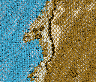
I am currently working up some Tenix LADS MKII lidar data over the Isles of Shoals off the coast of New Hampshire. I must say, the data set is quite impressive. Not only does the lidar bathymetry match very well with EM3002 multibeam bathymetry we have in the same area (initial comparison shows a mean difference of 0.6 m w/ a std: 0.3 m), but the seamless transition of the lidar data from water to land follows very closely the transition between the foreshore and the water (soundings are reduced to MLLW).
Here you can see the transition from depth soundings (blue) to terrain heights (brown) from the LADS lidar system. The flightlines are oriented north-northeast by south-southwest. NOAA chart 13283 is peeking out from behind the soundings. You can just see how the transition in sounding type roughly follows the foreshore line (MLLW) on the chart.
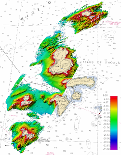
What does the bathymetry from the LADS MKII lidar look like? Here's a peak of some of the lidar bathy data (blue soundings only) gridded at a 4-meter resolution and displayed in Fledermaus. Sun illumination is from the northwest and the vertical exaggeration is 3. NOAA chart 13283 is in the background.

Friday, May 8, 2009
LIDAR view of the Golden Gate Bridge
The Seafloor Mapping Lab at the California State University in Monterey Bay has recently obtained a new vessel-mounted Lidar system for shoreline surveys. From their website:
Integration of this technology with their existing mapping systems allows for some pretty impressive data displays:
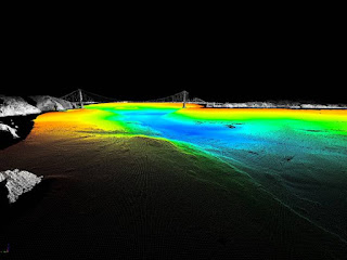 Combined bathy/topo DEM of the Golden Gate built by merging SFML's laser scanner (gray) and multibeam sonar (colored by depth) data (source: http://seafloor.csumb.edu/laserscanner.html)
They also have some pretty sweet 3D fly-throughs of the Golden Gate Bridge and the Los Padres Reservoir. I have included their Golden Gate Bridge fly-through below:
The high-resolution data set seen above was collected using SFML's new vessel-mounted mobile marine LIDAR system. Working with our industry partners, Riegl and Applanix, we have implemented an easily and rapidly deployable laser scanner capable of achieving decimeter accuracy with sub-meter resolution at a 1 kilometer range. This system gives SFML the ability to map the intertidal shoreline, offshore rocks and pinnacles and coastal features in unprecedented detail without the need for more costly airborne LIDAR surveys. The high spatial precision and accuracy of the system enable SFML to reliably monitor and quantify coastal erosion and landslide rates, bridge deformation, railway subsidence and coastal highway slippage through repetitive shoreline mapping surveys; information critical to coastal communities as they plan for climate change and sea level rise.
Integration of this technology with their existing mapping systems allows for some pretty impressive data displays:
 Combined bathy/topo DEM of the Golden Gate built by merging SFML's laser scanner (gray) and multibeam sonar (colored by depth) data (source: http://seafloor.csumb.edu/laserscanner.html)
They also have some pretty sweet 3D fly-throughs of the Golden Gate Bridge and the Los Padres Reservoir. I have included their Golden Gate Bridge fly-through below:
Sunday, March 8, 2009
Modeling a Lidar System: Part 1
Now that I am really starting to get into my research with lidar systems, I feel that it is important to understand as many of the intricacies and nuances of the system as possible, and how they interact with each other. Although I am certainly learning a lot from reading countless articles and texts, and having great directed study sessions with my chairs, I feel one of the best ways to learn is through a more experiential approach. Since I do not have full-fledged lidar system at my disposal to fly around with and image things (anyone offering?), I figure the next best thing I can do is theoretically model the system.
To get myself started, I found a paper by H. Michael Tulldahl and K. Ove Steinvall entitled: "Analytical waveform generation from small objects in lidar bathymetry," (App. Optics, v.38 n.6, 1999). The authors present a model to simulate received lidar waveforms in order to observe the influence of variously-shaped objects on the seabed. I am tweaking the modeled system parameters to match those of the systems I am working with, as well as the water-dependent parameters to match different water types. I am also not dealing with any objects on the seabed, and for now am assuming a flat bottom. I have only just started, so my model is nowhere near complete. Although this model is not the primary focus of my research, I see it as a way to help me understand not only what I am seeing in the data, but also predict features in the data that I might look for. Eventually I would like to have a user interface where I could simply select the lidar system and approximate water type (most likely based off Jerlov), and perhaps bed type and approximate roughness, and just hit "go!"
The model is currently in Matlab, though as it develops I may switch to a more object-oriented scripting language such as Python (I can hear Kurt applauding from here). The point is, models (and the more specifically, the development of models) can be a powerful learning tool. I wish that modeling itself (or at least an introduction to modeling) was taught as more of a core research tool, opposed to a special one.
Below is a snippet of some of the model output as it now stands. The top graph shows the volume backscattered power reaching the receiver. The middle graph shows the amount of power incident on the seabed (one-way travel), and the bottom graph shows the percentage of transmitted power returned to the receiver, all as a function of depth. In this case, the off-nadir angle of the laser is 0 degrees and I am looking only at the nadir beam. I am assuming pure seawater (just to make my initial attempts a little easier) and treating the water surface return of the green wavelength and the atmospheric loss as negligible.

Wednesday, October 29, 2008
Lidar data in Caris pt. 2: waveform view
I have been looking at more lidar data in CARIS today with one of my committee members and am now starting to really figure out how CARIS displays the data. In my previous post I mentioned that the peak with the green line represents the determined depth and the peak with the red line represents an "alternate depth." This "alternate depth" designation in CARIS is somewhat misleading, as this peak actually represents the small amount of energy from the green (532 nm) pulse that is reflected by the water surface. The reason that the peak appears larger, in some instances, than the bottom return is presumably due to the gain settings being amped up so a detection could be made.
Looking at the image below, this does seem to make sense. In this dataset, 3 peaks can clearly be seen. In CARIS, the 1064 nm and 532 nm returns are shown on the same graph, with the first x number of bins coming from the IR return, and the remaining bins coming from the green return. The first unmarked peak represents the IR return from the water surface. The red marked peak is the 532 nm surface return ("alternate depth") and the green marked peak is the 532 nm bottom return. If you look under the lidar tab, the depth for the "alternate depth" is 0.16 m, which becomes negative (out of the water) once a tide value is applied. I am assuming that this depth reading is due to the fact that the green surface return, though nominal, would still have a slight penetration through the water surface. It could also be related to the difference between the IR detected distance to the water surface and the green detected distance to the water surface.

Thursday, October 2, 2008
Lidar Data in CARIS HIPS and SIPS
The new version of CARIS HIPS and SIPS (v. 6.1) can now bring in SHOALS and LADS lidar data and waveforms for quality control and to merge it with multibeam data. The import procedure is pretty painless, though there still seem to be a few bugs to work out.
I tested it out with some LADS data I have from Portsmouth Harbor. You can see the selected data points highlighted in yellow in the plan view. The point highlighted in blue is the current "super-selected" point, and it is for this data point that CARIS will display the waveform. If you click either "next" or "previous" in the lefthand lidar menu, the "super-selected" point will move to the next yellow highlighted point and you can view the waveforms for each of the selected soundings.
The waveform box shows the surface and bottom returns for the green waveform. The green line represents the detected bottom depth for the waveform, while the red line represents a possible alternate depth. Unfortunately, there is no way to display axes (neither time nor intensity) or any type of scale on the waveform in order to get a better sense of what is being displayed. This is something CARIS will hopefully correct in later versions or hotfixes.


Tuesday, September 30, 2008
Lidar on Mars: The Movie
Kurt sent me a great movie clip showing an animation of the Optech lidar system on the Phoenix Mars Polar Lander and a series of false-color composite still frames.
You can really see the laser as it reflects off particles in the atmosphere. Note the rather large flash that shows up to the left of the laser. I am not sure what is going on there. Perhaps an accumulation of dust particles?
(if this plays really fast the first time, try playing it again. For some reason, the second time plays slow enough that you can see the flash)
Wednesday, July 23, 2008
Shoals 400 lidar data
Today I got my first glimpse of lidar data processing using Shoals NT, the Shoals 400 Hz Post-Flight Processing System. It took me a little time to muddle through everything and I am still not entirely sure what all the different functions do (even with a slightly out-of-date manual), but I am starting to get the hang of it. I am definitely itching to start really digging into this data.
Here is a screen shot of some Lake Tahoe data displayed in the software. You can see the overview area in the top left window and the zoomed in area in the box on the right. In both windows, lidar returns with a depth confidence of less than 50 are returned as no data (white). The rest of the returns are color-coded by depth. Land returns are brown. By clicking on individual soundings in the zoom window I can view more detailed information, including the full waveform.
 (click on the image for a larger version)
Friday, July 11, 2008
Lidar Data Organization in Google Earth
The USGS has really impressed me with their lidar data organization. You can view and download their data in a KML format using any KML viewer. One click on their data markers allows you to download the data in various formats (e.g. DEM, GeoTiff, XYZ, etc.) After playing around with it in Google Earth, I definitely think I will be following their example as a model for my own data organization.
Check it out for yourself here.
Here is a screen shot of the KML file from Biscayne Bay National Park displayed in Google Earth. The arrows represent areas of lidar data. The yellow dots are SCUBA dive site locations.

Check it out for yourself here.
Here is a screen shot of the KML file from Biscayne Bay National Park displayed in Google Earth. The arrows represent areas of lidar data. The yellow dots are SCUBA dive site locations.

Sunday, June 8, 2008
a simplified lidar waveform
Here is a simplified schematic of the green laser pulse waveform from lidar. Both surface return and bottom return times are picked at the half-peak amplitude. The volume backscatter is caused by the light reflecting off particles and colored dissolved organic material (CDOM) in the water column.
In reality, these curves would not be smooth but would actually be quite noisy. As I start to work with some of the lidar data, I will post more information about the waveforms.

In reality, these curves would not be smooth but would actually be quite noisy. As I start to work with some of the lidar data, I will post more information about the waveforms.

Friday, June 6, 2008
What is lidar?
Lidar: light detection and ranging (think sonar, only with light!)
There are both land- and water-based applications of lidar.
The basic principle of bathymetric lidar is that a laser mounted on an airplane or helicopter generates both a green (532 nm) and infrared (1064 nm) light pulse. The infrared pulse, which essentially has no attenuation in water, reflects off the air-sea interface and provides a surface return. The green pulse, which does attenuate, penetrates the water and reflects off the seabed giving a bottom return. The difference in travel time between the surface return and the bottom return can be used to estimate water depth. Because lidar is optical it is constrained to the photic zone and is heavily dependent on water clarity. Therefore, lidar typically will only work in 50 meters of water or less. A couple of the tech specs claim 70 meters, but this has yet to be actually acquired in the field. If I learned anything at all during this tech review, it is to take company technical specifications with a huge grain of salt!
Here is a nice little schematic of the green energy pulse that I modified from (Guenther 2001 [pdf]).
When the green energy pulse hits the water, a small portion of it reflects off the surface. The remainder penetrates the water column, where it is subjected to refraction, absorption, and scattering. When the light wave hits the seabed, it reflects back towards the laser and is again subjected to refraction, absorption, and scattering. Only about 4% of the incident green energy reaches the seafloor.
If you are interested in lidar, the Guenther chapter is a great introduction.

Subscribe to:
Comments (Atom)