It's finally happened. Barnes and Nobles is now offering free WiFi in all their stores.
http://www.barnesandnoble.com/help/cds2.asp?r=1&PID=27206
One of my favorite combinations (outside peanut butter and chocolate) is a good bookstore (avec cafe) and free wifi.

Friday, July 31, 2009
Tuesday, July 21, 2009
USGS Woods Hole: An Excellent Metadata Example!
Over the last couple years or so, I have become more and more concerned about metadata. Metadata is basically a file (txt, html, or xml) that accompanies a dataset and describes how, why, and when the data were collected, how they were processed, and who the primary contacts are. It can get more complicated, and there is also the matter of formats and whether or not it is compliant with the FGDC (Federal Geographic Data Committee) standards, but suffice to say the role of metadata is to give anyone reading it sufficient knowledge to be able to confidently use the data.
Good metadata is hard to find, and people routinely seem to underestimate its importance. Even if people do fill out metadata, they often skip a lot of important fields or simply do not include all the pertinent information (e.g. the tide station used to correct their data). What good is a multibeam dataset, for example, if I do not know how it was collected, if/how they corrected for tides and vessel motion, how they processed it, etc.? Oh sure, maybe you know what organization collected it, but what if they cannot remember? What if the main person responsible for that data no longer works there? A proper metadata file that accompanies the data will solve these issues.
Today I came across what I consider to be perhaps one of the best examples of metadata that I have seen. The metadata is for a multibeam dataset collected by the USGS in Woods Hole. All the pertinent fields are filled out, and for each section there is a point of contact listed. The reasons for the survey are given, as are the vessel used, the sonar used, how the sonar was mounted, etc. Not only did they specifically mention how they measured their vertical/horizontal accuracy and include an estimated uncertainty, but they include their tidal station information complete with NOAA tide station number so I can easily go and obtain the same tide record myself. What is most impressive, however, is that they list all their processing steps. They processed their data using SwathEd, a program developed at UNB that I am not familiar with. No problem though, because in the metadata, they actually give a numbered list of their processing steps complete with the command lines needed to do it myself! It is even broken up into editing that was done at sea, and the final editing steps undertaken to create the grids once they were back in the office.
Of course, no matter how good the metadata are, there is always room for some improvement. For example, it would be nice to see a separate ancillary data section perhaps, that lists the specific type and brand of IMU used, the type of CTD or sound velocimeter used, etc., along with manufacturer-stated (or observed) uncertainties.
Check out the USGS metadata, and of course the accompanying data, here: USGS Stellwagen Bank data. The data and metadata are all located under the GIS data links. The specific file I was looking at is here.
Here are some snippets of the metadata file to give you an idea (Note there are chunks of metadata skipped between snippets):
____________________________________________________
Good metadata is hard to find, and people routinely seem to underestimate its importance. Even if people do fill out metadata, they often skip a lot of important fields or simply do not include all the pertinent information (e.g. the tide station used to correct their data). What good is a multibeam dataset, for example, if I do not know how it was collected, if/how they corrected for tides and vessel motion, how they processed it, etc.? Oh sure, maybe you know what organization collected it, but what if they cannot remember? What if the main person responsible for that data no longer works there? A proper metadata file that accompanies the data will solve these issues.
Today I came across what I consider to be perhaps one of the best examples of metadata that I have seen. The metadata is for a multibeam dataset collected by the USGS in Woods Hole. All the pertinent fields are filled out, and for each section there is a point of contact listed. The reasons for the survey are given, as are the vessel used, the sonar used, how the sonar was mounted, etc. Not only did they specifically mention how they measured their vertical/horizontal accuracy and include an estimated uncertainty, but they include their tidal station information complete with NOAA tide station number so I can easily go and obtain the same tide record myself. What is most impressive, however, is that they list all their processing steps. They processed their data using SwathEd, a program developed at UNB that I am not familiar with. No problem though, because in the metadata, they actually give a numbered list of their processing steps complete with the command lines needed to do it myself! It is even broken up into editing that was done at sea, and the final editing steps undertaken to create the grids once they were back in the office.
Of course, no matter how good the metadata are, there is always room for some improvement. For example, it would be nice to see a separate ancillary data section perhaps, that lists the specific type and brand of IMU used, the type of CTD or sound velocimeter used, etc., along with manufacturer-stated (or observed) uncertainties.
Check out the USGS metadata, and of course the accompanying data, here: USGS Stellwagen Bank data. The data and metadata are all located under the GIS data links. The specific file I was looking at is here.
Here are some snippets of the metadata file to give you an idea (Note there are chunks of metadata skipped between snippets):
- Data_Quality_Information:
-
- Attribute_Accuracy:
-
- Attribute_Accuracy_Report: No attributes are associated with these data.
- Completeness_Report:
- These data were corrected for tidal elevation using the NOAA Boston tide gage. This assumes that the tidal elevation and phase are the same as Boston across the survey area. Further processing to correct for the spatial and temporal changes in tidal elevation across the survey area may be undertaken at a later time.
- Positional_Accuracy:
-
- Horizontal_Positional_Accuracy:
-
- Horizontal_Positional_Accuracy_Report:
- These data were navigated with a Differential Global Positioning System (DGPS); they are accurate to +/- 3 meters, horizontally.
- Vertical_Positional_Accuracy:
-
- Vertical_Positional_Accuracy_Report:
- These data have been corrected for vessel motion (roll, pitch, heave, yaw) and tidal offsets, and referenced to mean lower low water. The theoretical vertical resolution of the Simrad EM-1000 multibeam echosounder is 1 % of water depth, approximately 0.3 - 1.0 m within the study area.
____________________________________________________
- Process_Step:
-
- Process_Description:
- Data acquisition at sea
These multibeam data were collected with a Simrad EM1000 multibeam echo sounder mounted on the starboard pontoon of the Canadian Hydrographic Service Vessel Frederick G. Creed. The data were collected over four cruises carried out between the fall of 1994 and fall of 1998. Operation of the Simrad EM1000 was carried out by hydrographers of the Canadian Hydrographic Service. Data were collected along tracklines spaced 5-7 times the water depth apart at a speed of 10-14 knots. The frequency of the sonar was 95kHz. Sound velocity profiles were obtained and input into the Simrad processing system to correct for refraction. Navigation was by means of differential GPS.
- ____________________________________________________
- Process_Step:
-
- Process_Description:
- Final data processing and editing
Processing was carried out to further edit and correct the data and to produce final grids and images of the data. Processing and editing steps included:
1. Correct errors in soundings due to sound refraction, caused by variations in sound velocity profile, using the SwathEd refraction tool. These artifacts can be recognized in a cross-swath profile of a relatively flat patch of sea floor. When viewing the swath data across a profile, the sea floor will appear to have a "frown" or "smile" when in fact the data should be flat across the profile. Insufficient and/or erroneous sound velocity information, which is usually due to widely spaced or non-existent velocity profiles within an area, results in an under or over-estimate of water depth which increases with distance from the center of the swath. For a discussion of how this effect can be recognized in a swath bathymetric data file, see <
2. Remove erroneous soundings that were not edited in the field using the SwathEd program.
3. Correct the bathymetric data to mean lower low water by subtracting the observed tide at Boston, Massachusetts from the edited bathymetric soundings. This correction assumes that the tidal phase and amplitude are the same as Boston across the survey area.
Mean Lower Low Water (MLLW) tidal information was obtained from the NOAA tide server using tide station 8443970 located at Boston, MA (42 degrees 21.3 minutes N, 71 degrees 3.1 minutes W) (
Command line: binTide -year YYYY asciiTideFile BinaryTideFile
The program mergeTide brings the swath soundings to the MLLW vertical tidal datum:
Command line (tides): mergeTide -tide BinaryTideFile filename.merged Command line (navigation): mergeNav -ahead 5.379 -right 3.851 -below 4.244 filename (prefix only)
4. Create a 6-m grid of the bathymetric soundings for western Massachusetts Bay Quadrangles using the SwathEd routine weigh_grid.
Command line: weigh_grid -fresh_start -omg -tide -coeffs -mindep -2 -maxdep -800 -beam_mask -beam_weight -custom_weight EM1000_Weights -butter -power 2 -cutoff 12 -lambda 3 gridFile filename.merged
5. Convert binary bathymetric grid to ESRI ASCII raster format:
Command line: r4toASCII gridFile.r4
This creates a file called gridFile.asc.
Thursday, July 16, 2009
Image Processing in Matlab: Update 1: Filters
Okay, so I have been continuing to play around, trying to get my feet wet with image processing. I sort of jumped ahead here and begin fiddling with filters. Since I have the nadir artifact in my mosaic, I need to see if I can easily remove it.
I decided to use an adaptive filter since the noise I am most concerned is repetitive through the image (though not truly periodic as survey line spacing varies), so I do not need the same level of filtering over the whole image. I have been reading through the Matlab Image Processing documentation(pdf), and followed their directions for using "wiener2" which adaptively applies a Wiener linear filter to the image.
from the description under "help wiener2":
WIENER2 lowpass filters an intensity image that has been degraded by
constant power additive noise. WIENER2 uses a pixel-wise adaptive Wiener
method based on statistics estimated from a local neighborhood of each
pixel.
I used a 10x10 pixel neighborhood for filtering. Then, I ran the Sobel edge detect algorithm as described in my previous post. The results are below:
 on the left: orginal image on the right: wiener2 filtered image. Click to see full-size image so you can see the differences.
 The nadir artifacts are clearly less noticeable in the filtered image, and indeed the edge detect algorithm is now starting to pick up on the actual different patches of seafloor. The outline of the bright patch in the middle can now be seen.
I then increased the size of my filter to 20x20 pixels. Check out how well the edge detect performs now.


Beginning Image Processing in Matlab
I am starting to explore image processing in Matlab, and so far I am impressed with how easy it seems. I began with a 2000 x 2000 pixel gray scale image of a backscatter mosaic from EM3002 multibeam sonar data. I saved this image as a .tif and loaded it into Matlab using the 'imread' function. Once loaded, using "imshow" will display the image.
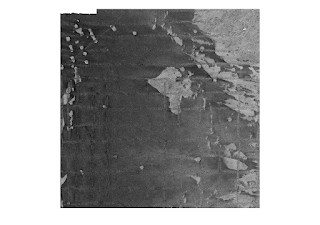
One of the first things I tried was the histogram function "imhist", to see how spread out my pixel values were between 0 - 255. Clearly my image does not make use of the full range of colors.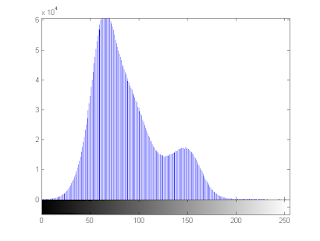 I then used "histeq" to stretch the intensity values between the full range of colors. Below are the resulting histogram and new higher contrast image.
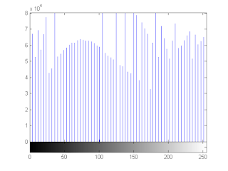
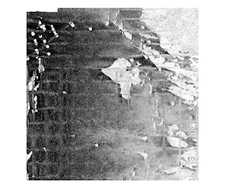 You can clearly see the artifacts from the nadir beam of the sonar where you get a brighter return. I figured this would be a good test of one of the edge detect algorithms to see if it picks them all out. I used the "edge" command and specified the Sobel method, leaving the threshold value blank. You can also specify a direction, however, I left it as the default, which looks for both horizontal and vertical edges. Here are the results:
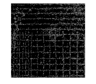 Pretty cool. It almost looks like a trackline map of the survey!

One of the first things I tried was the histogram function "imhist", to see how spread out my pixel values were between 0 - 255. Clearly my image does not make use of the full range of colors.
 I then used "histeq" to stretch the intensity values between the full range of colors. Below are the resulting histogram and new higher contrast image.
 You can clearly see the artifacts from the nadir beam of the sonar where you get a brighter return. I figured this would be a good test of one of the edge detect algorithms to see if it picks them all out. I used the "edge" command and specified the Sobel method, leaving the threshold value blank. You can also specify a direction, however, I left it as the default, which looks for both horizontal and vertical edges. Here are the results:
 Pretty cool. It almost looks like a trackline map of the survey!
Saturday, July 4, 2009
Daylilies in full bloom
After an exhausting roadtrip from KY back to NH, it was nice to come home and see the Daylilies in full bloom.

Blogger likes to resample the color scheme when it resizes the image to fit inside the blog post, so if you want to see the lilies in all their glory, be sure to click on the pic to see it full size:

Blogger likes to resample the color scheme when it resizes the image to fit inside the blog post, so if you want to see the lilies in all their glory, be sure to click on the pic to see it full size:
Subscribe to:
Posts (Atom)